Fifteen Eighty Four

“Fasten your seatbelts, we are expecting turbulence”.  On long-haul flights this is a routine announcement intended for the lay public, yet it conveys a deep-seated misconception about the nature of turbulence. The misconception is that atmospheric air motions are basically smooth (technically, “laminar”) occasionally interspersed with small embedded turbulent zones: the implication is that somehow the “smooth” and turbulent parts of the atmosphere are associated with distinct dynamics.  From there, it is a small step to develop separate scientific theories for each.  The imputation of distinct mechanisms to (apparently) distinct phenomena is a species of phenomenological fallacy as discussed in section 1.3 of [Lovejoy and Schertzer, 2013] – abbreviated WC below- and in another blog.   Not only is it responsible for erroneous interpretations of aircraft measurements, it has contributed to prolonging the life of an outdated picture of atmospheric dynamics.

Aircraft measurements are often our only direct source of data about the variability of the wind, temperature, humidity and other atmospheric variables in the horizontal direction.

The aircraft’s sudden “transitions from quiescence to chaos” – from apparently smooth to chaotic conditions – is a defining feature of the turbulent notion of “intermittency” (see fig. 1).  Although first described as “spottiness”, in laboratory flows [Batchelor and Townsend, 1949] it reflects to the ubiquitous property of the atmosphere to concentrate almost all its activity in regions occupying only a tiny fraction of the whole  – for example in storms and even in the centers of storms.  Since the 1980’s – and largely thanks to the development of the multifractal cascade models reviewed in WC – there has been dramatic progress in understanding intermittency.  It is now clear that by its very nature, turbulence is intermittent: as we zoom in we find violent regions in proximity to ones of relative calm.  Intermittency is evidenced by the occasional sharp “jumps” in the wind (fig. 1a), associated with high levels of turbulent energy flux (fig. 1b).  However, examination of the apparently calm regions shows that they also have embedded regions of high activity and as we zoom into smaller and smaller regions this strong heterogeneity continues in a scaling manner until we reach the dissipation scale. This explains why aircraft measurements of the wind invariably find roughly Kolmogorov type (i.e. turbulent) statistics even in apparently calm regions of the atmosphere.  This is hardly surprising since the ratio of the nonlinear terms in the dynamical equations to the linear (dissipative) terms (the Reynold’s number) is typically huge (≈10^¹²).  In any event, large scale regions of true laminar flow have yet to be documented by actual measurements. On the contrary, the multifractal, multiplicative cascade picture has been well verified even at large scales (see WC, ch. 4). Therefore, it would be a mistake to separate these regions of high and low “turbulent intensities” and associate them with different mechanisms.

Other blogs will discuss the consequences of the intermittency for classical notions and theories such as stable atmospheric layers and linear wave theories.  Here, I wish to report on a more immediate concern: the fact that aircraft measurements are often our only direct source of data about the variability of the wind, temperature, humidity and other atmospheric variables in the horizontal direction, yet the very turbulence they seek to measure, analyze and characterize modifies the trajectories and biases the results in ways that we are only now starting to understand.

There are two effects that we can note in fig. 1 a. The first is that although the aircraft stayed within 0.1% of a constant pressure level, that the altitude nevertheless is quite variable.  First, it is highly intermittent (fig. 1b) indeed it is fractal (even multifractal, [Lovejoy et al., 2009a]): although fortunately for the passengers at scales below 1 – 2 km, the aircraft inertia does tend to smoothed this out (otherwise in the small scale fractal limit, the accelerations would be infinite, [Lovejoy et al., 2004]!).
Second, in addition to its intermittency, the trajectory is not “flat”, but wanders up and down. Both effects bias the measurements.  We shouldn’t be surprised that the constant up and down intermittent “jiggling” of the aircraft leads to underestimates of the exponents characterizing the intermittency of the wind (and other fields), indeed, these are increased by roughly 0.02 to 0.03.  However, it turns out that these intermittency corrections turn out to be much less of a worry than the departures from constant levels. This is because the atmosphere is highly stratified, moving up and down a bit can lead to much larger variations in the wind than simply moving along in the horizontal direction. Due to this effect, exponents characterizing the mean wind fluctuations could be off by as much as 0.3.

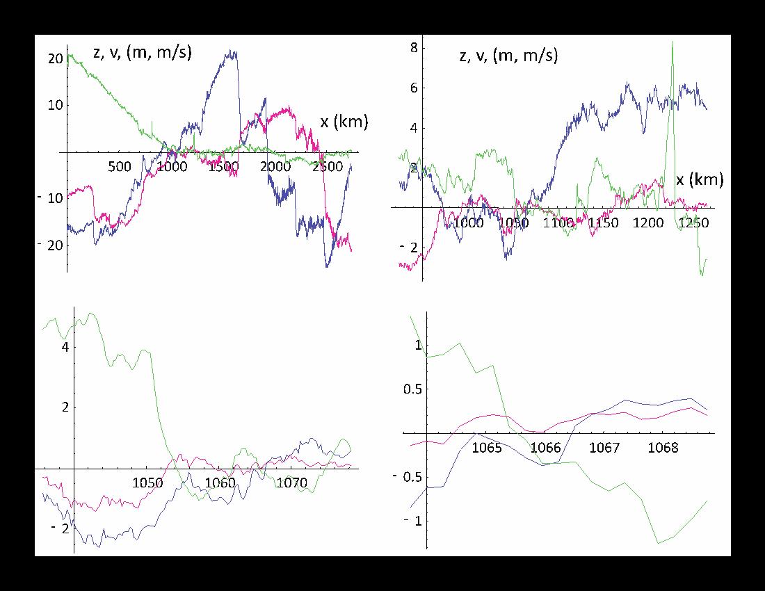
Fig. 1a: The trajectory (green) of a scientific aircraft (Gulfstream 4) following a constant pressure level (to within 0.1%), data at 1 s resolution (≈280 m). The red shows the variation in the longitudinal component of the horizontal velocity (in m/s, deviations from 24.5 m/s), and the blue is the transverse component (in m/s, deviations from 1.2 m/s). Moveing from upper left to right, top to bottom, we show three blowups by factors 8 in scale. Green shows the deviations of z from the 12 700m of the altitude of the aircraft, (in m) but divided by 8, 4, 2, 1 respectively (the overall trajectory thus changes altitude by over 160 m overall). This is for flight leg 15, but was typical. Reproduced from [Lovejoy et al., 2009a].

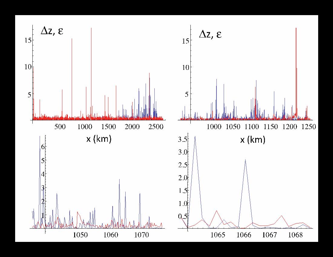
Fig. 1b: The figures corresponding to fig. 1a, but for the change in altitude (in m, red) and the turbulence energy flux (blue; the units are 4×10^-3 W/Kg). All except the upper left are multiplied by 40 to make them visible. The energy flux is estimated from the cube of the absolute wind gradient at the smallest scale.

Larger and larger atmospheric structures become flatter and flatter at larger and larger scales, but that they do so in a scaling (power law) way.  Contrary to the postulates of the classical 3D/2D model of isotropic turbulence, there is no drastic scale transition in the atmosphere’s statistics.   However, since the famous Global Atmospheric Sampling Program (GASP) experiment (fig. 2) there have been repeated reports of drastic transitions in aircraft statistics (spectra) of horizontal wind typically at scales of several hundred kilometers.  We are now in a position to resolve the apparent contradiction between scaling 23/9D dynamics and observations with broken scaling.  At some critical scale – that depends on the aircraft characteristics as well as the turbulent state of the atmosphere –  the aircraft “wanders” sufficiently off level so that the wind it measures changes more due to the level change than to the horizontal displacement of the aircraft.  It turns out that this effect can easily explain the observations.  Rather than a transition from characteristic isotropic 3D to isotropic 2D behavior (spectra with transitions from k^^-5/3 to k^^-3 where k is a wavenumber, an inverse distance), instead, one has a transition from k^^-5/3 (small scales) to k^^-2.4 at larger scales (fig. 2), the latter being the typical exponent found in the vertical direction (for example by dropsondes, [Lovejoy et al., 2009b]).

Since the 1980’s, the wide range scaling of the atmosphere in the both the horizontal and the vertical was increasingly documented; many examples are shown in WC, ch. 1.   By around 2010, the only remaining empirical support the 3D/2D model was the interpretation of fig. 2 (and others like it) in terms of a “dimensional transition” from 3D to 2D.  These interpretations were already implausible since a re-examination of the literature had shown that the large scales were closer to k^^-2.4 than k^^-3, as expected due to the “wandering” aircraft trajectories.  Finally, just last year, with the help of ≈14500 commercial aircraft flights with high accuracy GPS altitude measurements, it was possible for the first to determine the typical variability in the wind in vertical sections, and this was almost exactly the predicted 23/9=2.555… value: the measured “elliptical dimension” being ≈2.57.  It is hard to see how the 3D/2D model can survive this finding.

So next time you buckle up, celebrate the fact that the turbulence you feel is still stimulating scientific progress!

Fig. 2: Spectrum of the long haul aircraft flights from the GASP experiment. The lines with slopes -5/3 and -3 shows the predictions of the 3D/2D model; the -5/3 and -2.4 slope the prediction of the 23/9D model with aircraft “wandering” in the vertical. Reproduced from WC, fig. 2.10, adapted from [Gage and Nastrom, 1986].

References:

Batchelor, G. K., and A. A. Townsend (1949), The Nature of turbulent motion at large wavenumbers, Proceedings of the Royal Society of London, A 199, 238.

Gage, K. S., and G. D. Nastrom (1986), Theoretical Interpretation of atmospheric wavenumber spectra of wind and temperature observed by commercial aircraft during GASP, J. of the Atmos. Sci., 43, 729-740.

Lovejoy, S., and D. Schertzer (2013), The Weather and  Climate: Emergent Laws and Multifractal Cascades, 496 pp., Cambridge University Press, Cambridge.

Lovejoy, S., D. Schertzer, and A. F. Tuck (2004), Fractal aircraft trajectories and nonclassical turbulent exponents, Physical Review E, 70, 036306-036301-036305.

http://www.physics.mcgill.ca/~gang/eprints/eprintLovejoy/PREtraj.final36306-1.pdf

Lovejoy, S., A. F. Tuck, D. Schertzer, and S. J. Hovde (2009a), Reinterpreting aircraft measurements in anisotropic scaling turbulence, Atmos. Chem. Phys. Discuss., , 9, 3871-3920.

http://www.physics.mcgill.ca/~gang/eprints/eprintLovejoy/neweprint/acp-2008-0616-final.pdf

Lovejoy, S., A. F. Tuck, S. J. Hovde, and D. Schertzer (2009b), The vertical cascade structure of the atmosphere and multifractal drop sonde outages, J. Geophy. Res., 114, D07111, doi:07110.01029/02008JD010651.

http://www.physics.mcgill.ca/~gang/eprints/eprintLovejoy/neweprint/jgr.vertical.cascades.final.2008JD010651-2.pdf

Pinel, J., S. Lovejoy, D. Schertzer, and A. F. Tuck (2012), Joint horizontal – vertical anisotropic scaling, isobaric and isoheight wind statistics from aircraft data, Geophys. Res. Lett., 39, L11803 doi: 10.1029/2012GL051698.

http://www.physics.mcgill.ca/~gang/eprints/eprintLovejoy/neweprint/Pinel.GRL.2012GL051689.final2.pdf