Fifteen Eighty Four

Clouds come in a bewildering variety of sizes and shapes.  While they may all be fractal, some would require 3D shapes such as spheroids or ellipsoids to contain them while others – flat, elongated and perhaps wispy – might fit into thin 2D “sheet – like” containers.   The 3D-looking ones tend to be smaller while the 2D-looking ones tend to be larger: enormous flat “decks” of cirrus or stratus clouds are common.

With clouds, what one sees with the naked eye depends not only on the distribution of water droplets and ice particles but also on  the lighting, yet it is easy to imagine that other better defined atmospheric structures – such as regions above a certain temperature or wind threshold –  might be similarly shaped.  In classical turbulence theory, the structures of the atmospheric motions are called “eddies” and for over 40 years the prevailing statistical theory is precisely that the small eddies are 3D, whereas large ones are 2D.

But what is the real dimension of atmospheric motions?

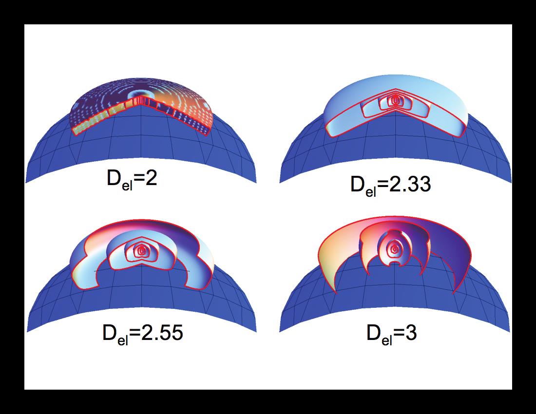
Fig. 1: A schematic showing average atmospheric structures as functions of scale for various elliptical dimensions (Del; reproduced from fig. 6.8 in [Lovejoy and Schertzer, 2013]). The different shells showing the average shape of “containers” of increasing size. The models vary from uniform thickness upper left, Del = 2, to three dimensional (lower right cut-off in the vertical to indicate the effect of the finite atmospheric thickness).

Thirty years ago, on the basis of balloon measurements and scaling symmetries, at two conferences, coauthor Daniel Schertzer and I made the audacious claim that they had the in-between “elliptical” dimension 23/9 = 2.555, [Schertzer and Lovejoy, 1983a], [Schertzer and Lovejoy, 1983b]. The year was 1983 and the nonlinear chaos and fractal revolutions were in full swing: we were invited to develop the idea further [Schertzer and Lovejoy, 1985]. To understand the claim, consider the schematic diagrams in fig. 1 illustrating the idea of “elliptical dimensions”.  Think of the cloud “containers” which bound the actual fractal clouds/eddies.  How do their volumes change as the horizontal lengths of the containers get larger?  For 3D clouds, the volumes would increase with the cube of the horizontal length while for 2D clouds, the thickness would not vary much with horizontal extent and the volume would only increase quadratically. The notion of elliptical dimension simply generalizes this: the container volume is the horizontal extent raised to the power D_el.  When D_el <3, the vertical grows less quickly than the horizontal so that the aspect ratio increases: fig. 1 shows how structures with D_el =23/9, become flatter and flatter at larger scales, yet never becoming 2D and how at small scales they become rounder and rounder while never becoming 3D.  The rational fraction 23/9 follows from dimensional analysis if the energy fluxes dominate the horizontal dynamics and buoyancy force variance fluxes dominate those in the vertical.

Back in 1983, the enthusiasm of the times smiled on this theory of anisotropic scaling turbulence.  But in the longer run, it came up against the meteorological community that had embraced Jules Charney’s theory of “quasi-geostrophic turbulence”.  This theory was based on the conventional (and ultimately flawed) assumption that small and large scales had totally different dynamics (with respectively 3D and 2D characters).  The ensuing thirty years is a classical story of seperate and unequal scientific development.  Eschewing fundamental questions such as the dimension of atmospheric motions, the meteorological community focused instead on the rapid development of numerical models.  In contrast the virtually unfunded 23/9 D model developed not only more slowly but rather in the nascent and separate nonlinear geophysics community.  It wasn’t until 2012 (see [Pinel et al., 2012], that it finally overcame the last argument in favour of geostrophic turbulence.  Today, the 23/9 D theory is the only one capable of explaining modern remote and in situ observations.  These developments are among the primary subjects of the book [Lovejoy and Schertzer, 2013] and more of this story was told in another blog on aircraft data.

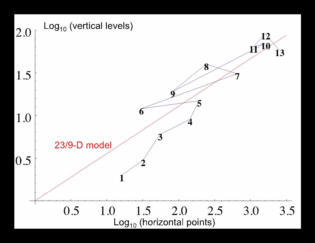
Fig. 2: The horizontal-vertical resolutions of numerical weather models, numbered chronologically; detailed in table 1. For models with several possible resolutions, the largest is used. Also shown is the theoretical relation predicted by the 23/9-D model: (vertical levels) = (horizontal points)5/9.

If reality is 23/9D and the numerical models are realistic, then the models should reflect this fact.  Indeed, detailed analyses of the internal statistical structure of the models confirms that they display the predicted types of multifractal cascades [Stolle et al., 2009]; but this only indirectly supports the 23/9D picture.  However, so far no one has noticed that the entire historical development of numerical weather models supports a 23/9 dimensionality!  Think of the containers.  For the model to be optimally adjusted so as to contain the largest eddies, its vertical extent (in model levels) should be close to the 5/9 power of the horizontal extent (in pixels) so that overall the number of degrees of freedom (model elements) is roughly the 23/9 power of the number of horizontal pixels.

In the developping of a numerical weather model, the horizontal resolution is generally fixed by practical (mostly computer) constraints, however some experimentation  is needed to determine the optimum number of vertical levels.  Therefore,  if we plot the number of vertical levels as a function of the number of horizontal points, we should expect it to at least roughly follow a 5/9 power law.  Fig. 2 – taken from an admittedly somewhat subjective sampling of historically significant models – confirms this idea surprisingly well.

Whatever one’s opinion of the 23/9 D picture of atmospheric motions, it has left it’s mark!

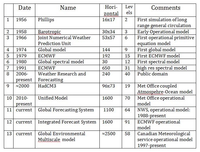
Table 1: Details on the models used in fig. 2; the left column numbers correspond to the numbers in the figure.

References

Lovejoy, S., and D. Schertzer (2013), The Weather and  Climate: Emergent Laws and Multifractal Cascades, 496 pp., Cambridge University Press, Cambridge.

Pinel, J., S. Lovejoy, D. Schertzer, and A. F. Tuck (2012), Joint horizontal – vertical anisotropic scaling, isobaric and isoheight wind statistics from aircraft data, Geophys. Res. Lett., 39, L11803 doi: 10.1029/2012GL051698.

Schertzer, D., and S. Lovejoy (1983a), Elliptical turbulence in the atmosphere, paper presented at Fourth symposium on turbulent shear flows, Karlshule, West Germany, Nov. 1-8, 1983.

Schertzer, D., and S. Lovejoy (1983b), On the dimension of atmospheric motions, paper presented at IUTAM Symp. on turbulence and chaotic phenomena in fluids, Kyoto, Japan.

Schertzer, D., and S. Lovejoy (1985), The dimension and intermittency of atmospheric dynamics, in Turbulent Shear Flow 4, edited by B. Launder, pp. 7-33, Springer-Verlag.

Stolle, J., S. Lovejoy, and D. Schertzer (2009), The stochastic cascade structure of deterministic numerical models of the atmosphere, Nonlin. Proc. in Geophys., 16, 1–15.