Fifteen Eighty Four

When we study Chapter 5, Exploring Relationships Between Two Variables, we like to have students read the article found at  http://www.nhs.uk/news/2009/10October/Pages/sweets-violence-link.aspx to prepare for a class discussion that involves several main points from the chapter.

The article describes a longitudinal study of 17,415 people.  The researchers noted whether the participants self-reported that had been convicted of committing a violent crime by the time they were 34 years old and whether or not they had eaten candy daily when they were 10 years old.  They also collected data when the participants were 5 years old to classify their early development and their parents’ style of parenting.  Overall, 69% of respondents who were violent by the age of 34 years reported that they ate candy daily during childhood. In addition, candy was eaten daily by 42% of those who were non-violent.  It is important to note that only 81, less than 0.5%, of the children in this study became violent offenders by the time they were 34 years old.  The newspaper summaries of the study indicated that candy consumption in children caused them to grow up to be violent criminals.

We use this article to make the following points that are related to the chapter.

• When dichotomous variables are involved in a correlation, the coding determines the sign of that correlation.

Based on the percentages, we know that 69% of respondents who were violent by the age of 34 years reported that they ate candy daily during childhood. In addition, candy was eaten daily by 42% of those who were non-violent.  If we had created two variables based on these percentages, VIOLENT (coded with 1 = had committed a violent crime by age 34 and 2 = had not committed a violent crime by age 34) and CANDY (coded with 1 = had eaten candy daily at age 10 and 2 = had not eaten candy daily at age 10), what would the sign of the correlation have been between the variables?  Because people who had been violent had also tended to eat candy daily and those who had not been violent had not tended to eat candy, in this case, high scores on one variable tend to correspond to high scores on the other variable and low with low, and we would expect a positive correlation.  In fact, if we calculate the Pearson correlation on the percentages, we have r = .26.  If the coding had been reversed for one of the variables, we would expect the sign, but not the magnitude of the correlation to change.

• When creating a clustered bar graph of the results based on the given percentages, the choice of axes is important.

Because we know that 69% of respondents who were violent by the age of 34 years reported that they ate candy daily, the horizontal axis needs to indicate whether or not the person ate candy, because that is the denominator of the given percentage.  The graph itself and the related Stata commands are given below.

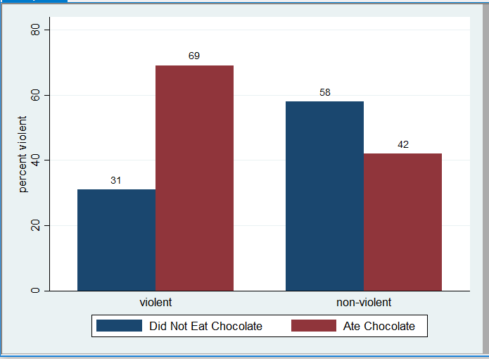
**label define violent 1 “violent” 2 “non-violent”

**label values violent violent

graph bar [fweight = freq], over(chocolate) asyvars percentage over (violent) blabel(total) ytitle(percent violent) ///

legend(label(1 “Did Not Eat Chocolate”) label(2 “Ate Chocolate”))

• The results are different when based on the percentages versus the frequencies.

Recall that the correlation between the two variables when based on the percentages was r = .26.  The authors indicated that only 81, less than 0.5%, of the children in this study became violent offenders by the time they were 34 years old.  That means that out of the 81 people who were violent offenders, about 56 (69%) ate candy daily and 25 did not.  Out of the 17334 people who were not violent offenders, about 7280 (42%) ate candy daily and 10,054 did not.  The correlation between the two variables when based on the frequencies is r = .04.  When taking into account the scarcity of violent offenders, we see that there is little or no relationship between the two variables.

• Causal conclusions have been made from observational data and this is problematic.

Although The Mirror probably sold more newspapers with the headline “Lots of sweets makes kids thuggish adults,” the study results do not support the claim that changing a person’s candy consumption at age 10 would change his or her violent behavior at age 34.  For example, if the parents are extremely permissive, that could be associated with a lot of candy consumption and also result in adults with less self-control who are more likely to commit violent crimes.  In that scenario, changing just one aspect of the permissive parenting by controlling candy consumption, probably will have little change in the likelihood of committing violent crimes.  When we ask our students to discuss, based on the results of this study, whether they would advise their parents to limit the candy consumption of their younger siblings, many who answer this question have a hard time limiting themselves to the results of the study.  They talk about how candy causes cavities and is not healthy and should be avoided.