Fifteen Eighty Four

When the International Meteorological Organization defined the first climate normal from 1900 to 1930, the belief was that the climate was constant, that the newly defined climate “normal” would provide a close approximation to the climate.   Today, we still use the 30 year “normal” period – referring now to 1960-1990 – but we acknowledge that it is not immutable, that even without anthropogenic effects, due to natural causes, that the climate changes.   But what then is the climate and what is the difference between the climate and the weather?  Mark Twain once quipped: “Climate lasts all the time and weather only a few days” (see the Quote Investigator for more of the history on this theme).  This is close to the popular dictum: “the climate is what you expect, the weather is what you get” [Heinlein, 1973].  Since most people “expect” averages, this concurs with the reigning idea that the climate is a kind of “average” weather.  Similarly, the use of Global Climate Models (GCM’s) to predict the climate is based on the idea that for given boundary conditions (solar output, atmospheric composition, volcanic eruptions, land use), that “the climate is what you expect”.

While all this sounds reasonable, it turns out that it is not based on analysis of real world data.  In recent papers “What is climate?” and “The climate is not what you expect” ([Lovejoy, 2013], [Lovejoy and Schertzer, 2013]) we used a new kind of “fluctuation analysis” to show that – at least up to 100,000 years – that that there are not two, but rather three atmospheric regimes each with different types of variability.  In between the weather and the climate, there is a new intermediate “macroweather” regime.   The time scale characteristic of the weather regime is about 10 days, it is determined by the lifetime of planetary sized structures, itself determined by the (solar forced) energy flux.  The time scale of the climate regime is determined by the scale at which slow climate processes begin to dominate the weather processes which become weaker and weaker at longer scales.  In the industrial period, the latter are dominated by anthropogenic effects and the transition scale is about 30 years, in the preindustrial period, the forcing is smaller and it is closer to 100 years.

What does it mean to define a regime by its type of variability?  An illustration makes it intuitive.  Consider fig. 1 which shows examples from weather scales (0.067 s, 1 hour resolution, bottom two), macroweather (20 days, second from the top) and climate (1 century, top).  For the middle two, the daily and annual cycles were removed and for each, 720 consecutive points are shown so that the differences in the characters of each regime are visually obvious.  The bottom two weather curves – whose characters are very similar to each other – “wander” up or down, resembling drunkard’s walks, typically increasing over longer and longer times periods.  In the second from the top, the macroweather curve has a totally different character: upward fluctuations are typically followed by nearly cancelling downward ones (and visa versa).  Averages over longer and longer times tend to converge, apparently vindicating “the climate is what you expect” idea: we anticipate that at decadal or at least centennial scales that averages will be virtually constant with only slow, small amplitude variations.  However (top) the century scale climate curve displays again a weather-like (wandering) variability. Although this plot shows temperatures, other atmospheric fields (wind, humidity, precipitation, etc.) are similar (although for these fields there are no high quality paleo proxies).

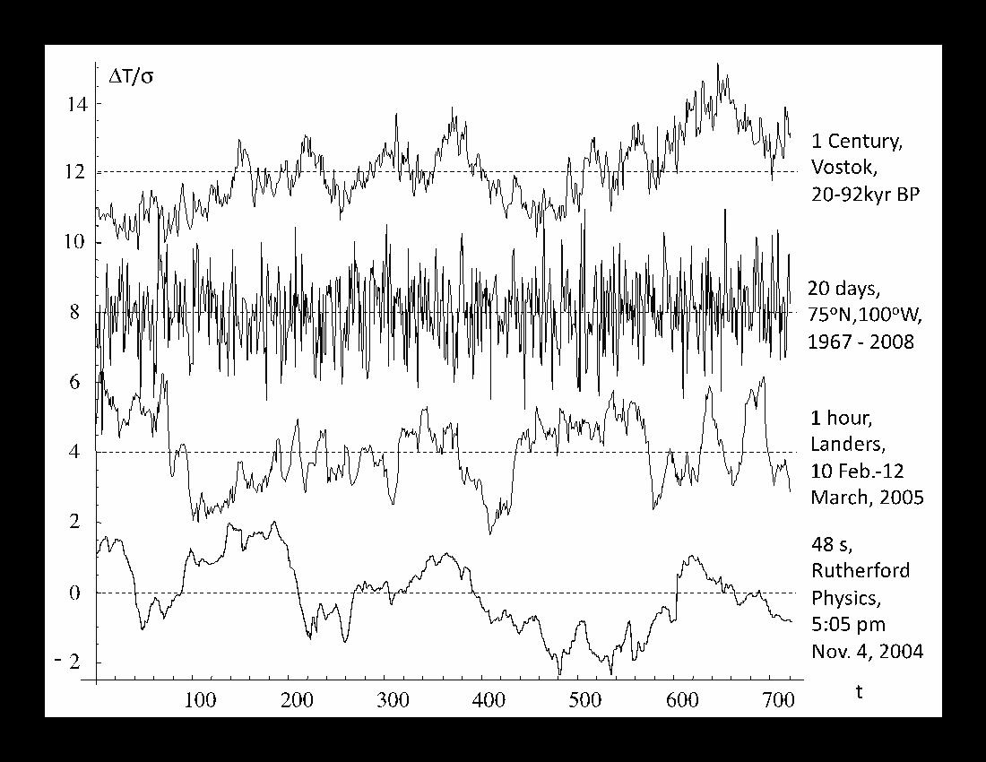
Fig. 1: Dynamics and types of scaling variability: Representative temperature series from weather, macroweather and climate (bottom to top respectively). Each sample is 720 points long and was normalized by its standard deviation (bottom to top: 0.35o C, 4.48o C, 2.59 o C, 1.39 o C, dashed lines indicate means). The resolutions are 0.066 s, 1 hour, 20 days and 1 century, the data are from, Montreal Canada (the roof of the physics building at McGill), Lander Wyoming, the 20th Century reanalysis and Vostok (Deuterium paleotemperatures, Antarctic) adapted from [Lovejoy, 2013].

There are thus three qualitatively different regimes, a fact was first recognized in the 1980’s and that has been confirmed several time since, but whose significance has not been appreciated [Lovejoy and Schertzer, 1986], [Pelletier, 1998], [Huybers and Curry, 2006].  The old analyses were based on analyzing temperature differences and spectra, and these suffered from various technical limitations and from difficulties in interpretation.  The new technique works by defining fluctuations over a give time interval by the difference of averages over the first and the second halves of the interval (“Haar” fluctuations); it is thus very easy to interpret.  In the “wandering” weather and climate regimes, the averaging in the definition isn’t important: fluctuations are essentially differences.  In the cancelling “macroweather” regime, the differences aren’t important, the fluctuations are essentially averages.  Whereas in the weather and climate regimes, fluctuations tend to increase with time scale, in the macroweather regime, they tend to decrease.  For example, over GCM grid scales (a few degrees across), the average fluctuations increase on average up to about 5^oC until about 10 days.  Up until about 30 years they tend to decrease to about 0.8^o C, and then – in accord with the amplitude and time scale of the ice ages – they increase again up to about 5^o C at ≈100,000 years (fig. 2).  In macroweather, averages converge: “macroweather is what you expect”.  In contrast, the “wandering” climate regime is very much like the weather so that – at least at scales of 30 years or more – the climate is “what you get”.   Conveniently, we see that the choice of 30 year time period to define the climate normal can now be justified as the time period over which fluctuations are the smallest.

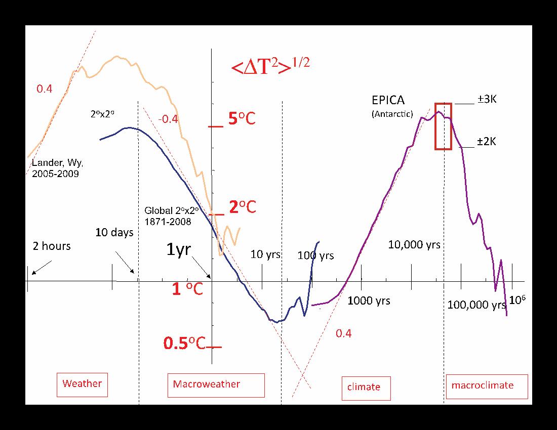
Fig. 2: This shows the typical (Haar) fluctuations for the Lander data (upper left), and paleo Antarctic data (from the EPICA core, near and similar to the Vostok core). Also shown is the globally averaged (at 2o resolution) fluctuations from the Twentieth century reanalysis. The various regimes are shown, along with power law (straight) reference lines with the slopes as indicated.

In a nutshell, average weather turns out to be macroweather – not climate – and climate refers to the slow evolution of macroweather.  This evolution is the result of external forcings (solar, volcanic etc.) coupled with natural (internal) variability: i.e. forcings with feedbacks.  In the recent period, we must add anthropogenic forcings.

Why “macroweather”, and not “microclimate”? It turns out that when GCM’s – which are essentially weather models with extra couplings (to oceans, sea ice etc.) are run in their “control” modes (i.e. with constant atmospheric composition, solar output, no volcanoes etc.) – that fluctuation and other analyses show that they well reproduce both the weather and the macroweather types of wandering and canceling behaviours, so that macroweather is indeed long term weather.  To obtain the climate they must at least include new climate forcings, but probably also new internal climate mechanisms; a recent fluctuation study shows that the multicentennial variability of GCM simulations over the period 1500-1900 are somewhat too weak [Lovejoy et al., 2012].

(this blog post is adapted from “Macroweather, not climate, is what you expect” posted on Climate Etc. in January 2013)

References

Heinlein, R. A. (1973), Time Enough for Love, 605 pp., G. P. Putnam’s Sons, New York.

Huybers, P., and W. Curry (2006), Links between annual, Milankovitch and continuum temperature variability, Nature, 441, 329-332 doi: 10.1038/nature04745.

Lovejoy, S. (2013), What is climate?, EOS, 94, (1), 1 January, p1-2.

http://www.physics.mcgill.ca/~gang/eprints/eprintLovejoy/neweprint/Macroweather.EOS.17.10.12.pdf

Lovejoy, S., and D. Schertzer (1986), Scale invariance in climatological temperatures and the spectral plateau, Annales Geophysicae, 4B, 401-410.

http://www.physics.mcgill.ca/~gang/eprints/eprintLovejoy/neweprint/Annales.Geophys.all.pdf

Lovejoy, S., and D. Schertzer (2013), The climate is not what you expect, Bull. Amer. Meteor. Soc., (in press).

http://www.physics.mcgill.ca/~gang/eprints/eprintLovejoy/neweprint/climate.not.13.12.12.pdf

Lovejoy, S., D. Schertzer, and D. Varon (2012), Do GCM’s predict the climate…. or macroweather?, Earth Syst. Dynam. Discuss., 3, , 1259-1286 doi: 10.5194/esdd-3-1259-2012.

Pelletier, J., D. (1998), The power spectral density of atmospheric temperature from scales of 10**-2 to 10**6 yr, , EPSL, 158, 157-164.